About this theme: bootstrap-blogdown

Posted on April 1, 2020 | 3 minute read

The theme on this website is called bootstrap-blogdown and is available on GitHub. It is an adaption of another Hugo theme called monopriv written by Sai Karthik (see GitLab). bootstrap-blogdown is a responsive, simple, yet element theme built using Bootstrap 4.4.1 CSS (hence the bootstrap) and is specially adapted for blogdown.

The theme has code formatting and highlighting to match that of RStudio’s basic HTML knitted documents. It natively supports MathJax therefore allowing complicated LaTeX (you can see for yourself in the Advanced Maths section below). The theme has been configured to deploy on Netlify with ease (blogdown’s preferred deployment platform) and has at least one user actively using it and being willing to maintain it (both cases being me…).

The winning YAML

Yihui Xie is owed a great thanks for creating both bookdown and blogdown. The two were always designed to integrate, but I do not think he drives home this point enough. blogdown with its ability to support proper mathematical numbering and its generally more robust HTML is a huge step up from the regular knitr offering. It is very easy to change from knitr by specifying in a (Rmd) YAML output: bookdown::html_fragment2. This also works excellently with blogdown. Below is my “winning” YAML for blogdown.

---
title: "About this theme"
author: "Jed Stephens"
date: 2020-04-01T21:00:00-00:00
categories: ["R"]
draft: true
tags: ["R", "bootstrap-blogdown", "monopriv"]
output: bookdown::html_fragment2
---

That test document

When you start a blogdown site it comes with a basic test document. That document, demonstrating how bootstrap-blogdown makes it appear, is below. An additional section shows off MathJax

Simple formatting

This is an R Markdown document. Markdown is a simple formatting syntax for authoring HTML, PDF, and MS Word documents. For more details on using R Markdown see http://rmarkdown.rstudio.com.

You can embed an R code chunk like this:

summary(cars)
##      speed           dist       
##  Min.   : 4.0   Min.   :  2.00  
##  1st Qu.:12.0   1st Qu.: 26.00  
##  Median :15.0   Median : 36.00  
##  Mean   :15.4   Mean   : 42.98  
##  3rd Qu.:19.0   3rd Qu.: 56.00  
##  Max.   :25.0   Max.   :120.00
fit <- lm(dist ~ speed, data = cars)
fit
## 
## Call:
## lm(formula = dist ~ speed, data = cars)
## 
## Coefficients:
## (Intercept)        speed  
##     -17.579        3.932

Advanced Maths

$α + 2 β - \frac{1}{4} = 5$

Including Plots

You can also embed plots. See Figure 1 for example:

par(mar = c(0, 1, 0, 1))
pie(
  c(280, 60, 20),
  c('Sky', 'Sunny side of pyramid', 'Shady side of pyramid'),
  col = c('#0292D8', '#F7EA39', '#C4B632'),
  init.angle = -50, border = NA
)

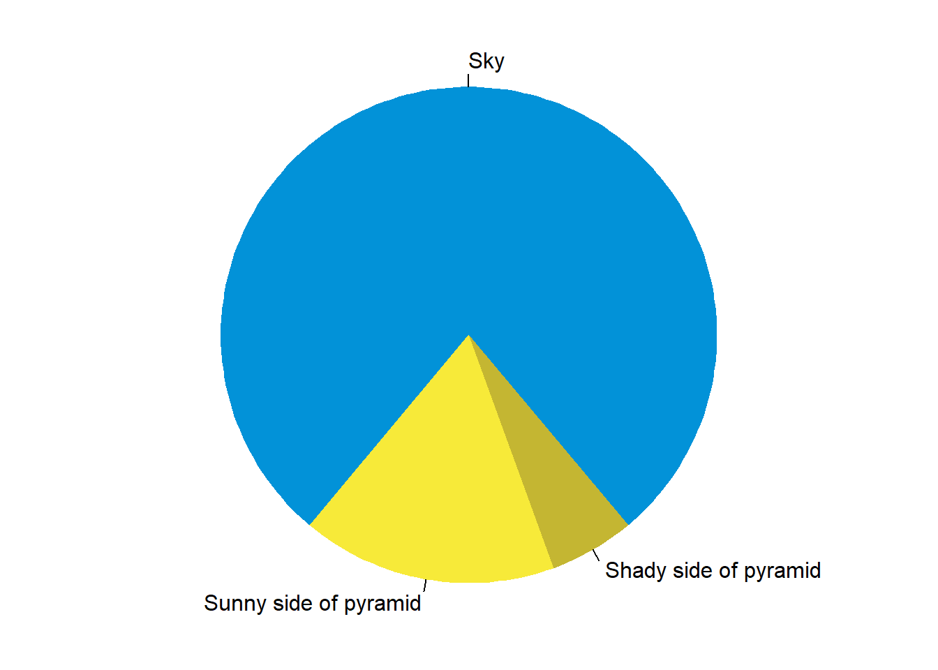
Figure 1: A fancy pie chart.

Share via

Tags:R
	  bootstrap-blogdown
	  monopriv